Animation Target Constraint

One common task game developers come across when using animated characters is to modify them in real-time in order to satisfy a given task. More particularly, re-using the same grab/take animation or push/punch/kick animation to target a specific object is a feature every programmer want and may have to implement.

When dealing with targets in animation, the first word that came into our mind is Inverse Kinematic (IK). And actually, that is a good start to tackle our problem. Indeed, for instance when a character has to grab an item, IK automatically find rotations and positions of the elbow and shoulder (can be more than that) so that the hand reach the target.

Let’s now define our problem more accurately. At a given frame of one animation, we want some body part of our character to reach a given target. As I like to consider an animation as a time function instead of a function of frame, we define $t_t$ our target time and $p_t$ the position of the given target.

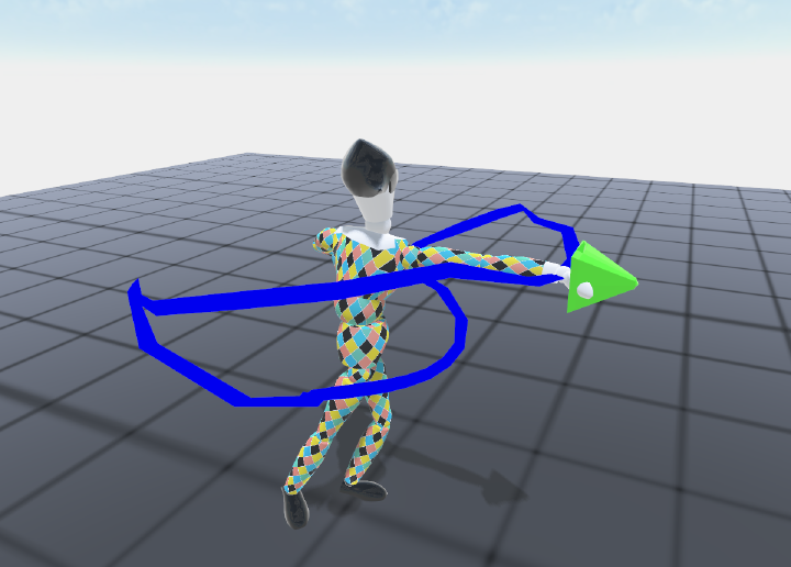
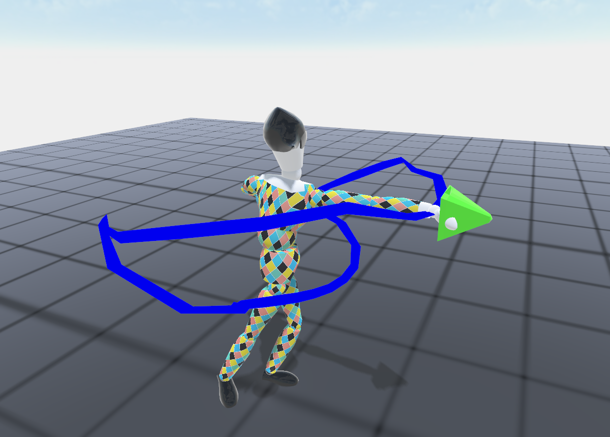
For a given bone, let’s say the hand, we compute its trajectory $p(t)$ or ${p_i}$ (discretized) during the whole animation. One could say that our problem is solved as we just have to call our IK solver at time $t_t$ so that $p(t_t) = p_t$. However, this solution while satisfying our constraint, induce a high discontinuity in the animation. Moreover, the character’s hand reach the target at the given frame without actually taking the trajectory to reach it as the rest of the animation remains unchanged. Our goal is then to change the overall hand motion so that it feels like the character aims to reach our target. One formulation of this problem is to also impose that while satisfying the target constraint, our initial animation remains as consistent as possible with respect to the original. This can be formulated as an as-rigid-as-possible (ARAP) deformation of the hand trajectory. While it was first used to deform 3D models, this paper used the same principle but for bones trajectories by noticing each point of one trajectory could be expressed in a local frame of defined by its neighbours:

$$ \forall i, p_i = p_{i-1} + \alpha_i \vec{A_i} + \beta_i \vec{B_i} $$

$$ \text{with } \vec{A_i} = \frac{p_{i+1} - p_{i-1}}{\left \lVert p_{i+1} - p_{i-1} \right \rVert} $$

This formulation translates the fact that $p_i$ can be expressed in a frame in which the frontal vector $\vec{A_i}$ and left vector $\vec{B_i}$ are contained in the $\hat{ p_{i-1}p_ip_{i+1}}$ plane, with $p_i$ being expressed with respect to its neighbors. Using simple trigonometry it is quite simple to compute $\alpha_i$ and $\beta_i$:

$$ \alpha_i = dot(p_i - p_{i-1}\vec{A_i}) $$

$$ \beta_i = \left \lVert cross(p_i - p_{i-1}\vec{A_i}) \right \rVert $$

Finally, we can deduce:

$$ \vec{B_i} = \frac{p_{i} - p_{i-1} - \alpha_i\vec{A_i}}{\beta_i} $$

Using this characterization of each point of the bone’s trajectory with respect to its neighbors, we seek to conserve each original $\alpha_i$ and $\beta_i$ when deforming the trajectory to address the $ p(t_t) = p_t $ constraint. Let’s consider that $p(t_t) = p_k$ for $k \in [1:n]$. We then compute the new bone trajectory as an optimization process minimizing the cost function $L_i$:

$$ L_i(p_0,…,p_n) = \sum\limits_j {\left\lVert (\alpha^{init}_j,\beta^{init}_j) - (\alpha_j,\beta_j) \right\rVert}^2 + \gamma {\left\lVert p_k - p_t \right\rVert}^2 $$

Using a gradient descent method we can update the ${p_i}$ trajectory at each step of the optimization process in which: $\forall j, p_j = p_j -\epsilon\nabla L_i(p_0,…,p_n)_j$.