An Introduction to Physically Based Rendering

Jan 1, 0001

This tutorial is inspired from https://learnopengl.com/PBR/Theory and adapted for the ray-tracing course available here.

Introduction

A big challenge in computer graphics is to design shading models mimicking real-life lighting behaviour while allowing intuitive control of object materials. This control is crucial for artists who are creating assets that have to be integrated in a rendering pipeline. For real-time applications like video games, the question of computation time and memory cost is also essential; such models must be flexible enough and allow affordable approximations.

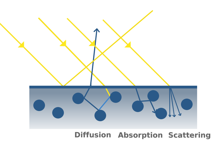
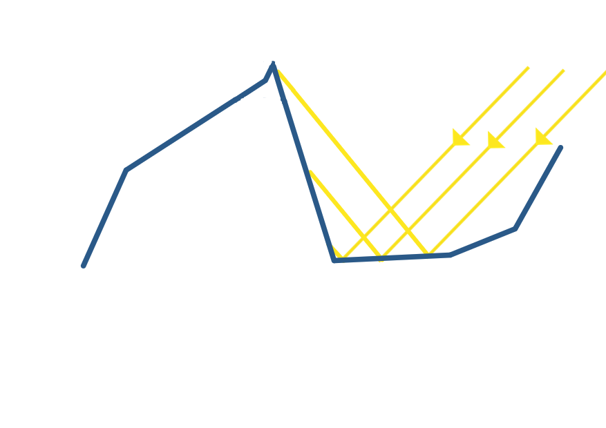
In this tutorial, we are interested in Physically Based Rendering (PBR) models which aim at simulating light behaviour in a more realistic way, approximating light related equations (models like the Phong model are very simplistic in comparison). One important aspect of those models is their energy conservative property stating that when interacting with a surface, the amount of outgoing light is equal to the amount of incoming light. More precisely, the amount of light absorbed, scattered and diffused by object surfaces is equal to the amount of light hitting the surface. The figure below illustrates these phenomena.

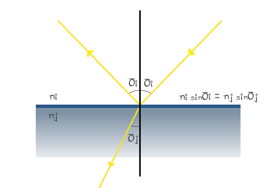
Simulating this behaviour is highly correlated with how we represent object surfaces. Indeed, light interaction with object surfaces is modeled by the Snell-Descartes law which describes how incident light gets refracted and reflected on a flat surface.

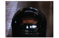
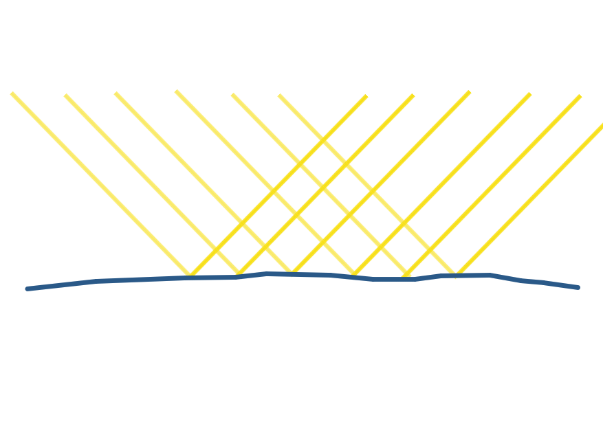
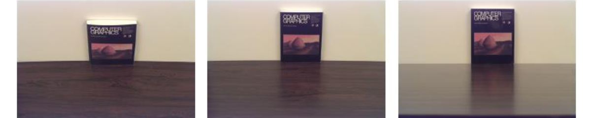
However, in practice object surfaces are not completely flat, some are rougher than others. This is something noticeable in real life, especially when you look at specular reflection on different objects. More precisely, rough surfaces tend to produce blurred reflections while smooth surfaces behave like mirrors.

Rough Surface	Smooth Surface
Rough Surface	Smooth Surface

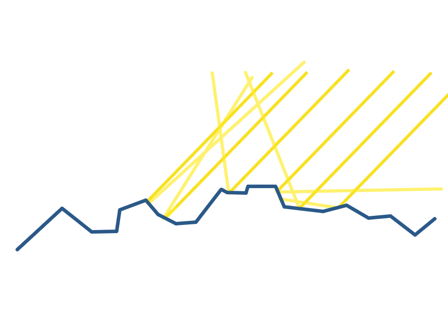
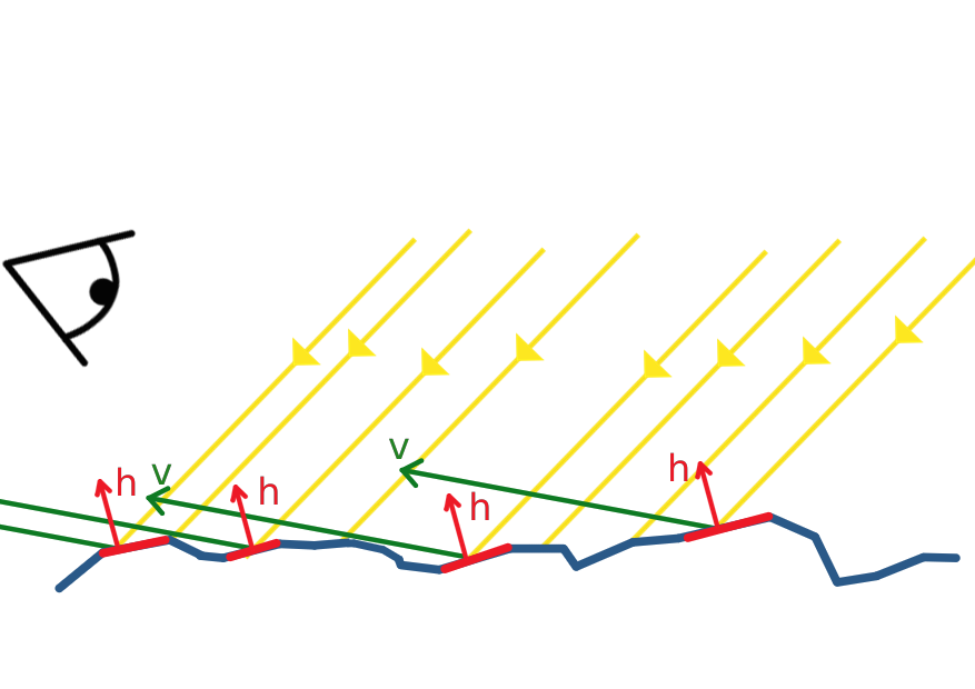
Thus, the microfacet model was introduced and defines a surface by a continuous sequence of flat micro-surfaces that might be oriented differently, simulating the smooth vs rough aspect of macro-surfaces. The roughness property of a material plays a meaningful role in light behavior as it controls the amount of light that gets reflected and refracted as well as the direction of outgoing light.

Rough Surface	Smooth Surface

Light Equation

Having stated all this principles, our main goal remains unchanged, compute the color received by the eye (camera) for each pixel of the output image displayed on our screen. More specifically, we are interested in the color and intensity of light that either gets directly reflected from the surface to the eye or that gets refracted and then re-emitted by the object through diffusion (considering that all the light that gets absorbed is lost). On the other hand, in this tutorial we neglect the effect of scattering which gives more realistic results (especially useful when rendering skin) but is more costly to compute.

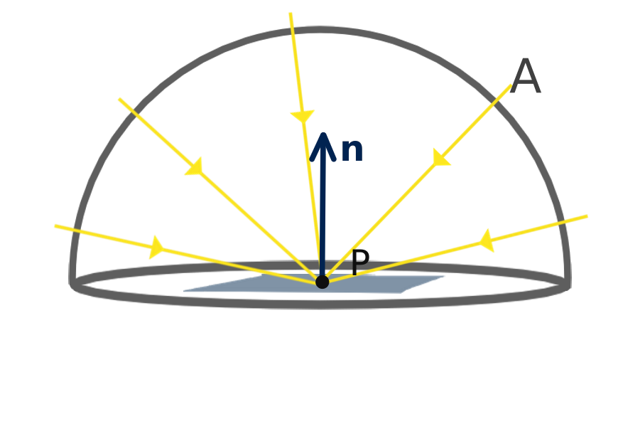
The amount of light that gets into a specific direction from a given point on an object surface is governed by laws of physics and more specifically it is given by the reflectance equation:

$$ L_o(p,v) = \int_A f_r(p,l,v,\alpha_p) L_i(p,l)(n \cdot l)dl $$

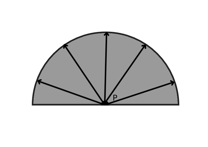
Where $p$ is the point of interest on the object surface (receiving light), $v$ the view direction from $p$ to the eye, $l$ the incident light direction, $\alpha_p$ the surface roughness at point $p$, $L_o$ the output light radiance (stored as a RGB color) perceived by our eye from $p$, $L_i$ the incident light radiance (also stored as a RGB color) gathering at $p$ from direction l, $f_r$ a function controlling the amount of light reflected to direction $v$ with respect to the material property at $p$ and $A$ the hemisphere surrounding $p$ on which we integrate all incoming light directions.

In this tutorial, we further restrict incoming light sources to a given number of point light sources. Thus, the integral over $A$ can be transformed into a sum over the different light sources.

$$ L_o(p,v) = \sum_l f_r(p,p-c_l,v,\alpha_p) L_i(p,p-c_l)( n \cdot \frac{(c_l-p)}{\left\lVert c_l - p \right\rVert}) $$

The incoming reflectance $L_i(p,p-c_l)$ equals to the intensity of the light source $I$, multiplied by its color $C$, and weighted by an attenuation factor which depends on the distance to the source. In our case, we will consider that the intensity of light decrease with the square distance to the source:

$$L_i(p,p-c_l) = \frac{IC}{{\left\lVert p - c_l\right\rVert}^2} $$

The Bidirectional Reflective Distribution Function (BRDF)

The only unknown left is the $f_r$ function that controls the amount of reflected light with respect to materials properties. This function is called a BRDF which stands for Bidirectional Reflective Distribution Function. Several functions were proposed to simulate real-life materials behavior, all of them respect the energy conservation law, meaning that the amount of outgoing light do not exceed the amount of incoming light and above all the later is divided between reflected and refracted light. Another important property of the BRDF functions is that there are intresectly symmetric with respect to incoming and outgoing light because of the principle of reversibility of light. In our case, we will use the Cook-Torrance BRDF model composed of a diffuse and a specular part:

$$f_r = k_d f_l + k_s f_c$$

where $k_d$ is the amount of refracted light that gets re-emitted and $k_s$ the amount of reflected light with:

$$ k_d = 1 - k_s $$

The $f_{l}$ function is the Lambertian diffusion distribution (which corresponds to the diffuse part of the Phong model). It considers that the diffused light is equally spread on all direcion: $$ f_l = \frac{C}{\pi} $$ Where C is the albedo of the object surface at point $p$. We can notice that the dot product between the normal and the light direction is done outside this function and is still present in the sum of in going contribution. $\pi$ is a normalization factor which accounts for the fact that we integrate ingoing light over the hemisphere at point $p$.

At this point it is important to mention that we must differentiate between two type of material: metals and dielectric (non metal) materials. Indeed, while dielectric materials diffuse light, it is not the case of metals that absorb all refracted light. As a consequence, $k_d = 0$ for metals (with $k_s \leq 1$ because light still get refracted).

On the other side the $f_c$ is composed of two terms:

$$f_c = \frac{DG}{4(l \cdot n)(v \cdot n)}$$

with D called the Normal Distribution Function and G the Geometry function. Additionally, $k_s = F$, where $F$ is the Fresnel term describing the amount of light that gets refracted on a more macroscopic scale with respect to the view direction. The Fresnel term results from an equation that is not easy to solve, however it can be approximated using the Fresnel-Schlick approximation:

$$ F_{Schlick}(h, v, F_0) = F_0 + (1 - F_0) (1 - (h \cdot v))^5 $$

With $F_0$ being the base reflectivity of the material and $h = \frac{l + v}{\left\lVert l + v \right\rVert}$ the half vector which corresponds to the normal one facet must have to directly reflect the light into the eye.

This equation tells us that when $h$ and $v$ are perpendicular the amount of reflected light is at its maximum, in other words reflections occurs more at grazing angles. This effect is especially noticeable on puddles or wooden surfaces when looking from a top view or from a grazing angle.

$F_0$ is computed as the amount of reflected light at normal incidence where $v$ and $l$ are collinear. It is important to note that this equation can only be applied to dielectric materials, especially because metallic materials absorb all refracted light. However, as $F_0$ for dielectric materials is usually low and high for metallic materials, a common approximation is to use a common average $F_0$ for dielectic materials and the metal color as $F_0$ for metallic materials. This is plausible because metallic $F_0$ are tinted and give to metals their color. Furthermore, following the metallic workflow we will consider that being metallic or dielectric is not a binary feature, meaning that one material can be sem-metallic with its metalness varying from $0$ to $1$.

NOTE: One might notice that $h$ is replaced by $n$ in the original equation. This is perfectly right in a macroscopic point of view. However, in our case we look at reflections in a microscopic scale, meaning that the normal of the surface is determined by microfacet normals. Additionally the only case where the light is reflected into our eye is when $n = h$ which justify our use of h in this case. This property is further used to approximate the BRDF final expression.

Fresnel coefficient length computed on our test scene (see below). The final amount has been remapped for visualisation purpose.

Let us describe the microfacet model in more details and focus on the roughness parameter that plays a role in the amount of reflected light. More concretely, this parameter describes the amount of micro-facet that are aligned in the same direction; in particular, rough surfaces have a chaotic orientation distribution while smooth surfaces facets are oriented in a single direction (the normal).

As microfacets represent the surface of the object, their orientation directly affects the direction of reflected light. That’s why smooth surfaces typically behave like mirrors while reflections appear blurrier on rough surfaces.

We can now describe the role of the Normal Distribution Function D and the Geometric function G. D represent the amount of microfacet that are aligned with the half vector $h$. This is the same as computing the amount of reflected light rays that are collinear to the view vector $v$.

In our case, we chose the GGX distribution function as NDF:

$$D = NDF_{GGX TR}(n, h, \alpha) = \frac{\alpha^2}{\pi((n \cdot h)^2 (\alpha^2 - 1) + 1)^2}$$

GGX Normal Distribution Function computed on our test scene with varying roughness (left: rough surface. right: smooth surface)

This function behaves like a diract when $\alpha = 0$ (smooth surface) and becomes flatter and flatter when $\alpha$ increases until it reaches a constant function $\frac{1}{\pi}$. That is why this formula produces small rounded highlight on smooth surfaces which are completely spread across the object on rough surfaces.

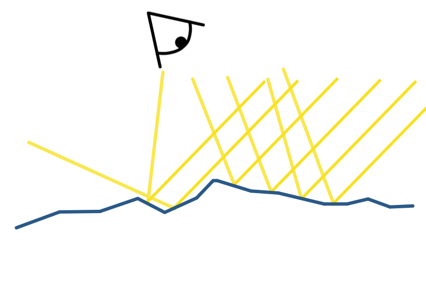
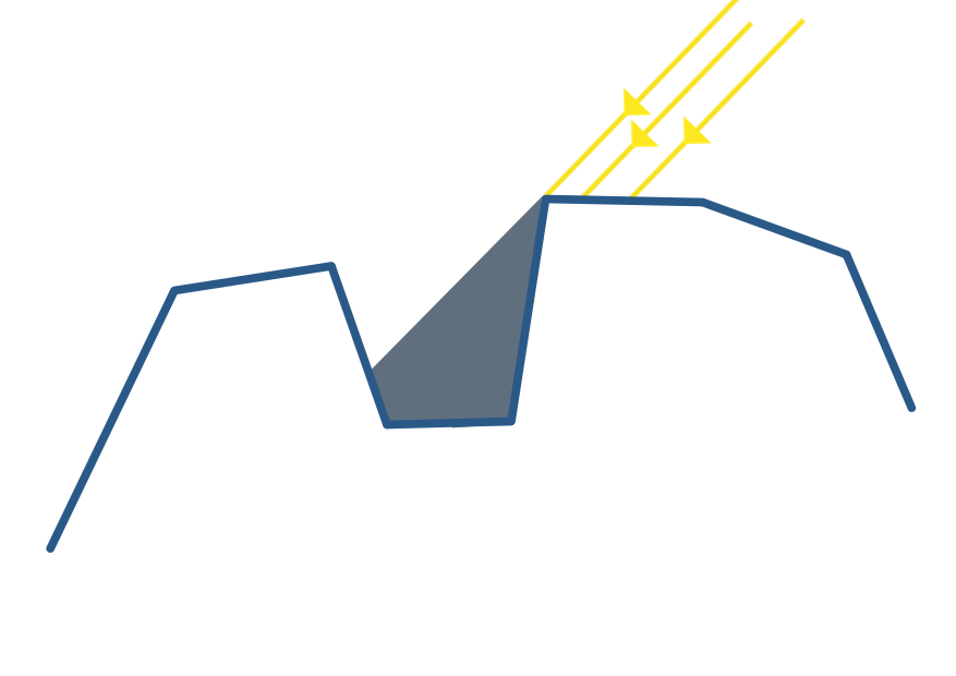
The Geometric function simulates two phenomena that occurs between micro-facets namely obstruction and shadowing. In the two cases, either the incoming light cannot reach some micro-facets because there are in the shadows of others (shadowing) or reflected light is blocked by other facets (obstruction).

Shadowing	Masking

Therefore, some amount of reflected light is “lost” and this is exactly the information given by the Geometric function. In our case we chose the Schlick-GGX approximation:

$$ G_S(n, v, k) = \frac{n \cdot v}{(n \cdot v)(1 - k) + k } $$

Taking into account the two effects:

$$ G(n,v,l,k) = G_S(n, v, k) G_S(n, l, k) $$

This function intuitively models the fact that at grazing angle with respect to the normal, either incoming light rays of reflected rays have a chance to collide with other facets. This probability is gets higher when the roughness of the surface increases, which is pretty intuitive because the micro-facet gets more chaotic and do not face a single direction.

Geometry function computed on our test scene (left: rough surface. right: smooth surface).

In this tutorial we made choices for approximation functions but several others can be found in the literature (see References at the bottom of the page), I invite you to take a look at BRDF comparison articles.

Coding Time

We are now ready to dive into the code. The base code can be found here. First, lets go back to our main function. We are working inside a fragment shader displaying a simple quad perfectly fitting our window. For each pixel we cast rays from a virtual camera to the current pixel whose screen coordinates are given by the in variable $fragCoord$.

in vec2 fragCoord;
void main()
{   
    Ray ray = generatePerspectiveRay(fragCoord);
    outColor = vec4(trace(ray),1);
}

Inside the fragment shader, I passed the view matrix $V$ of the trackball that is available from the transform.py file and used it to move the camera. Notice the inverse operator applied on V as we want to recover the position of the camera in world space.

uniform mat4 V;
Ray generatePerspectiveRay(in vec2 p)
{
    // p is the current pixel coord, in [-1,1]
    float fov = 30; // Half angle
    float D = 1./tan(radians(fov));
    mat4 inv_view = inverse(V); // Get the matrix of the trackball

    vec3 up = vec3(0,1,0);
    vec3 front = vec3(0,0,-1);
    vec3 right = cross(up,front);
    return  Ray((inv_view*vec4(0,0,-D,1)).xyz,mat3(inv_view)*normalize(p.x*right + p.y*up*aspectRatio + D*front));
}

Next we declare two new structures: the HitSurface structure containing a ray-scene intersection point, the surface normal at this point as well as its material properties expressed as a PBRMat. As mentioned above these materials contain roughness and metallic properties. We also add an ambient occlusion property which is used when computing an ambient lighting term in the rendering loop.

struct PBRMat
{
    vec3 color;
    float roughness;
    float metallic;
    float ao;
};

struct HitSurface
{
    vec3 hit_point;
    vec3 normal;
    PBRMat material;
};

Back to the trace function. We declare $accum$ as the color of the pixel that is incremented at each ray bounce, the $mask$ variable indicates the intensity of the current ray which gradually decrease at each bounce. For each step we compute the intersection between the ray and the objects in the scene and store the nearest intersected object (with a positive distance) in the $io$ variable.

The material used for the intersected object is chosen with respect to its index which is used to sample from an array of materials. We then compute the normal and the local illumination of the object at the intersection point inside the directIllumination function. The reflection intensity factor $c_{refl}$ is updated inside this function. Note, that the reflected ray origin is slightly shifted in the normal direction to avoid wrong self intersection. This tip is also applied when computing the shadow ray.

vec3 trace(in Ray r)
{
    vec3 accum = vec3(0.0f);
    vec3 mask = vec3(1.0f);
    int nb_refl = 2; // Bounce number
    float c_refl = 1.0f;
    Ray curr_ray = r;
    for(int i = 0 ; i <= nb_refl ; i++)
    {
        ISObj io = intersectObjects(curr_ray);
        if(io.t >= 0)
        {
            PBRMat mat = pbr_mat[io.i];

            HitSurface hs = HitSurface(curr_ray.ro + io.d*curr_ray.rd, computeNormal(io,curr_ray),mat);               

            vec3 color = directIllumination(hs,curr_ray,c_refl);
            accum = accum + mask * color;
            mask = mask*c_refl;
            curr_ray  = Ray(hs.hit_point + 0.001*hs.normal,reflect(curr_ray.rd,hs.normal));
        }
        else
        {
            break;
        }
    }

    return accum;

}

Inside the directIllumination function, we iterate through each light of the scene and determine if the current intersection point is in the shadow of an object (which can be it self) by casting a ray in the direction of the light. If the intersection point is actually lighted, we compute its radiance inside the PBR function. Otherwise we assign an ambient color weighted by the ambient occlusion factor of the material. Finally we update the reflection intensity factor by computing the length of th Fresnel term.

vec3 directIllumination(in HitSurface hit,in Ray r,inout float refl)
{

    vec3 color = vec3(0);
    for(int i = 0 ; i < light_nbr ; i++)
    {
        Ray l_ray = lightRay(hit.hit_point,lights[i]);
        l_ray.ro = hit.hit_point + 0.001*hit.normal;
        ISObj io;
        io = intersectObjects(l_ray);
        float d_light = lightDist(hit.hit_point,lights[i]);

        if(io.t < 0 || (io.t >= 0 && (io.d >= d_light)))
        {
            color += PBR(hit,r,lights[i]);
        }
        else
        {
            color +=  vec3(0.03) * hit.material.color * hit.material.ao;
        }


        vec3 Ve = normalize(r.ro - hit.hit_point);
        vec3 H = normalize(Ve + l_ray.rd);
        refl = length(fresnelSchlick(max(dot(H, Ve), 0.0),  mix(vec3(0.04), hit.material.color, hit.material.metallic)))*hit.material.ao;
    }

    return color;
}

struct Light 
{
    int type; // 0 dir light, 1 point light
    vec3 dir; // directionnal light
    vec3 center; // point light
    float intensity; // 1 default
    vec3 color; // light color
};

Ray lightRay(in vec3 ro, in Light l) //computes ro to light source ray
{
    if(l.type == 0)
        return Ray(ro,normalize(l.dir));
    else if(l.type == 1)
        return Ray(ro,normalize(l.center - ro));

    return Ray(ro,vec3(1));
 }

float lightDist(in vec3 ro, in Light l) //computes distance to light
{ 
    if(l.type == 0)
         return DIST_MAX;
    else if(l.type == 1)
        return length(l.center - ro);

    return DIST_MAX;
}

Next, it is time to actually implement the PBR direct illumination function approximating the light equation. This is done in two steps. We first compute the ambient term and the material $F_0$. We then compute the normal of the surface at the intersection point, the view vector, the half vector, the light intensity and direction and pass them to the computeReflectance function inside of which we compute the actual output radiance.

vec3 PBR(in HitSurface hit, in Ray r , in Light l)
{
    vec3 ambient = vec3(0.03) * hit.material.color * (1.0 - hit.material.ao);
    //Average F0 for dielectric materials
    vec3 F0 = vec3(0.04);
    // Get Proper F0 if material is not dielectric
    F0 = mix(F0, hit.material.color, hit.material.metallic);
    vec3 N = normalize(hit.normal);
    vec3 Ve = normalize(r.ro - hit.hit_point);

    float intensity = 1.0f;
    if(l.type == 1)
    {
        float l_dist = lightDist(hit.hit_point,l);
        intensity = l.intensity/(l_dist*l_dist);
    }
    vec3 l_dir = lightRay(hit.hit_point,l).rd;
    vec3 H = normalize(Ve + l_dir);
    return ambient + computeReflectance(N,Ve,F0,hit.material.color,l_dir,H,l.color,intensity,hit.material.metallic,hit.material.roughness);
}

We then define all the BRDF functions we mentionned above:

float DistributionGGX(vec3 N, vec3 H, float roughness)
{
    float a      = roughness*roughness;
    float a2     = a*a;
    float NdotH  = max(dot(N, H), 0.0);
    float NdotH2 = NdotH*NdotH;

    float nom   = a2;
    float denom = (NdotH2 * (a2 - 1.0) + 1.0);
    denom = PI * denom * denom;

    return nom / denom;
}

float GeometrySchlickGGX(float NdotV, float roughness)
{
    float r = (roughness + 1.0);
    float k = (r*r) / 8.0;

    float nom   = NdotV;
    float denom = NdotV * (1.0 - k) + k;

    return nom / denom;
}

float GeometrySmith(vec3 N, vec3 V, vec3 L, float roughness)
{
    float NdotV = max(dot(N, V), 0.0);
    float NdotL = max(dot(N, L), 0.0);
    float ggx2  = GeometrySchlickGGX(NdotV, roughness);
    float ggx1  = GeometrySchlickGGX(NdotL, roughness);

    return ggx1 * ggx2;
}

vec3 fresnelSchlick(float cosTheta, vec3 F0)
{
    return F0 + (1.0 - F0)*pow((1.0 + 0.000001/*avoid negative approximation when cosTheta = 1*/) - cosTheta, 5.0);
}

Finally, we compute the outgoing radiance as the product of the incoming radiance, the BRDF terms and the dot product between the normal and the light direction.

vec3 computeReflectance(vec3 N, vec3 Ve, vec3 F0, vec3 albedo, vec3 L, vec3 H, vec3 light_col, float intensity, float metallic, float roughness)
{
    vec3 radiance =  light_col * intensity; //Incoming Radiance

    // cook-torrance brdf
    float NDF = DistributionGGX(N, H, roughness);
    float G   = GeometrySmith(N, Ve, L,roughness);
    vec3 F    = fresnelSchlick(max(dot(H, Ve), 0.0), F0);

    vec3 kS = F;
    vec3 kD = vec3(1.0) - kS;
    kD *= 1.0 - metallic;

    vec3 nominator    = NDF * G * F;
    float denominator = 4 * max(dot(N, Ve), 0.0) * max(dot(N, L), 0.0) + 0.00001/* avoid divide by zero*/;
    vec3 specular     = nominator / denominator;


    // add to outgoing radiance Lo
    float NdotL = max(dot(N, L), 0.0);
    vec3 diffuse_radiance = kD * (albedo)/ PI;

    return (diffuse_radiance + specular) * radiance * NdotL;
}

And that’s it, we set up everything to compute a more realistic shading of our scene, you can already produce new raytraced results using this setup.

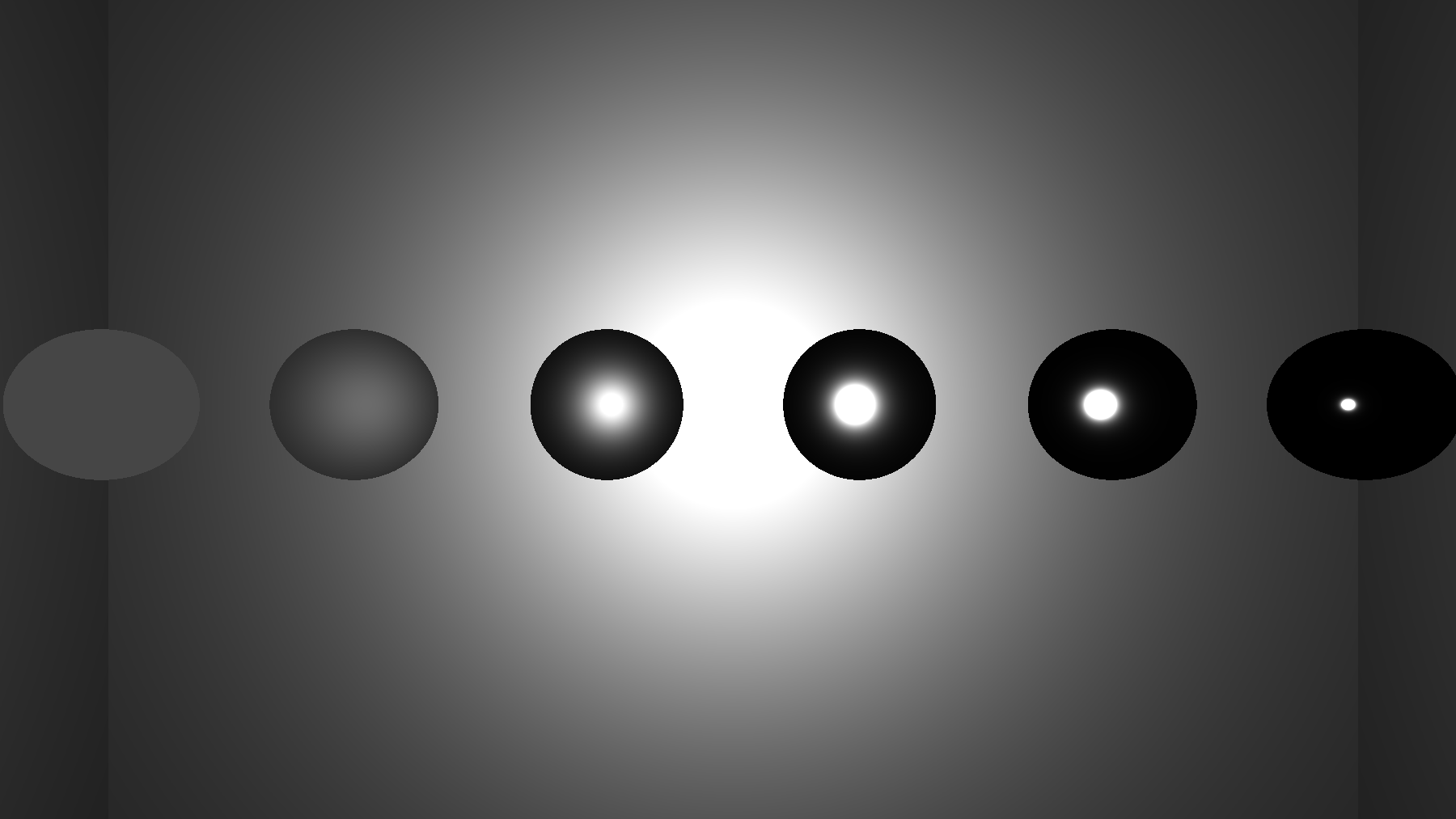
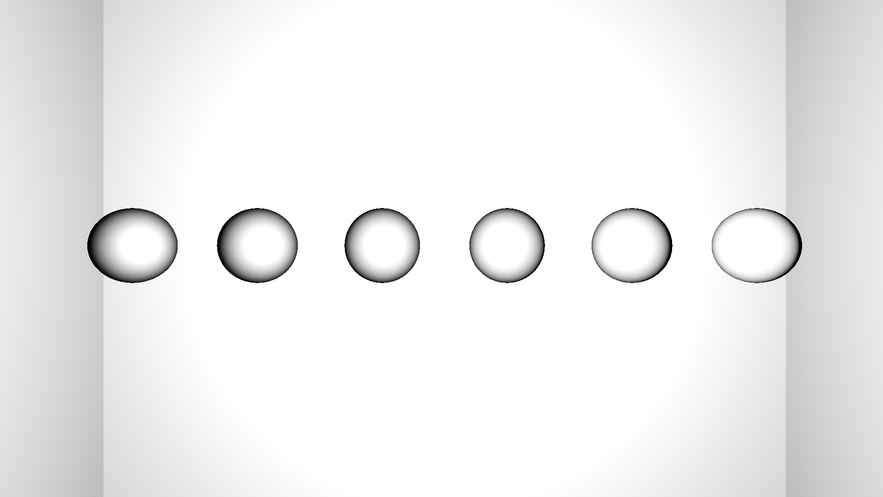
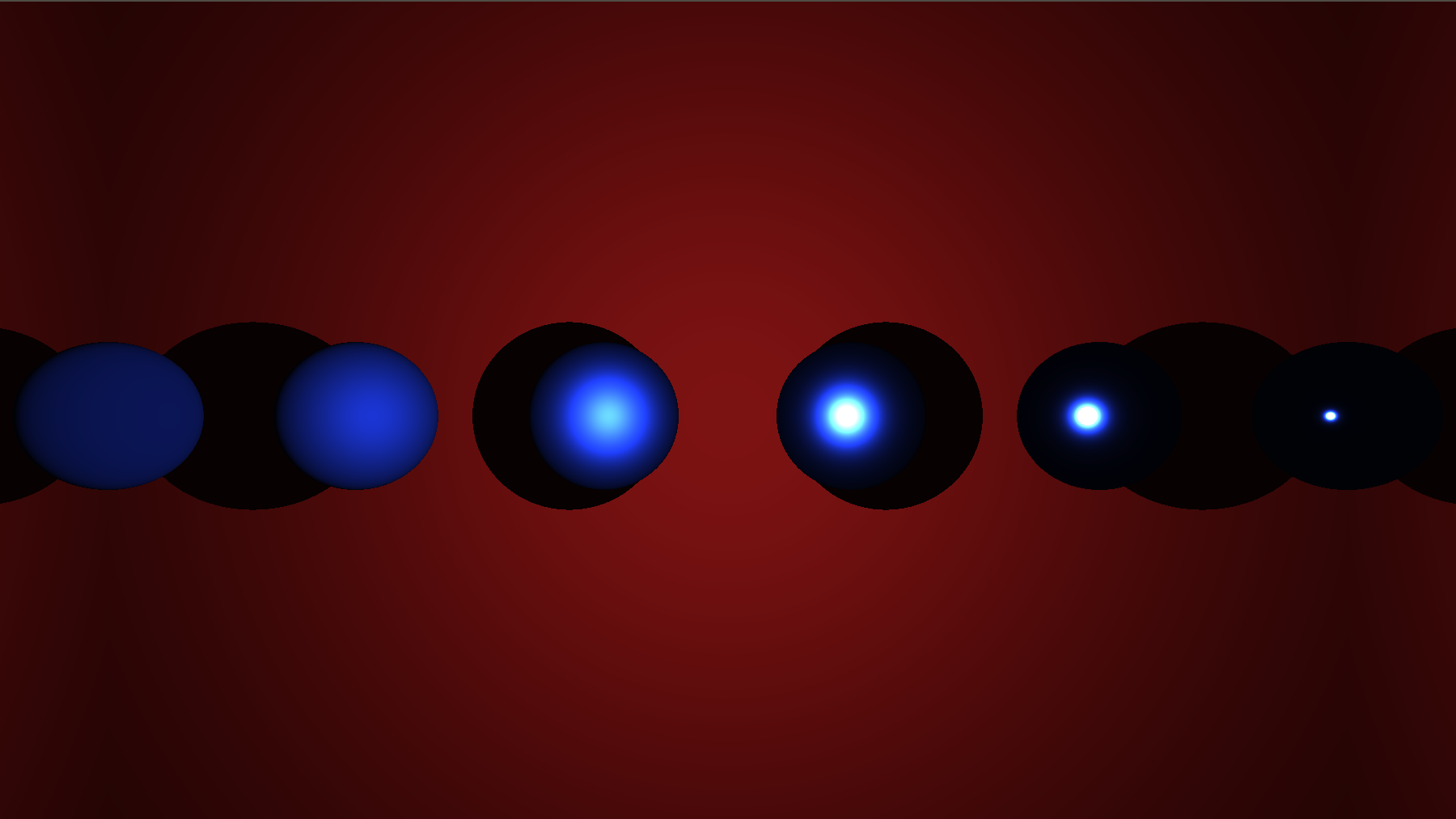
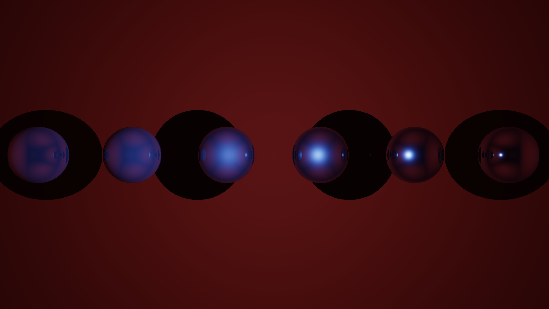
Below, are rendering examples of the same scene with varying materials. It contains a single white point Light of intensity $I = 40$ and located at (0,0,0). Left to right spheres roughness are 1, 0.9, 0.7, 0.5, 0.3, 0.1 with (.1,.2,.8) as color and are located at (2.5,0,-2), (1.5,0,-2), (0.5,0,-2), (-0.5,0,-2), (-1.5,0,-2) and (-2.5,0,-2) with a radius of 0.3.

Dielectric materials without reflection (metalness = 0)

Dielectric materials with reflection (metalness = 0)

Metallic materials without reflection (metalness = 1)

Metallic material with reflection (metalness = 1)

One last step: HDR and Gamma correction

So far we are able to render scenes in a more realistic way. Still, you can notice that if you choose a high intensity for your lights, the results also gets highly saturated, which is already the case in the above examples. This situation is to be expected because radiance can have value bigger than 1. Consequently, we need to find a way to account for High Dynamic Range (HDR) of radiance and process the computed values such that everything is remapped between 0 and 1. I won’t enter into details here as it is not the subject of this tutorial. We basically use the Reinhard operator to correct our input colors, remapping them inside the $[0;1]^3$ space with the function $C = \frac{C}{C+1}$.

Finally, we also need to take into account the color shift that screens produce in response to color values and depending on what we call their gamma value defining this response. Hence, we proceed to a gamma correction of the output colors which rectifies the shift. Again this will be covered in another tutorial, however be careful that this gamma value depends on the monitor configuration you are using.

vec3 trace()
{
    vec3 accum = vec3(0.0);
    ...

    //HDR
    accum = accum / (accum+ vec3(1.0));
    //Gamma
    float gamma = 2.2;
    accum = pow(accum, vec3(1.0/gamma));
}

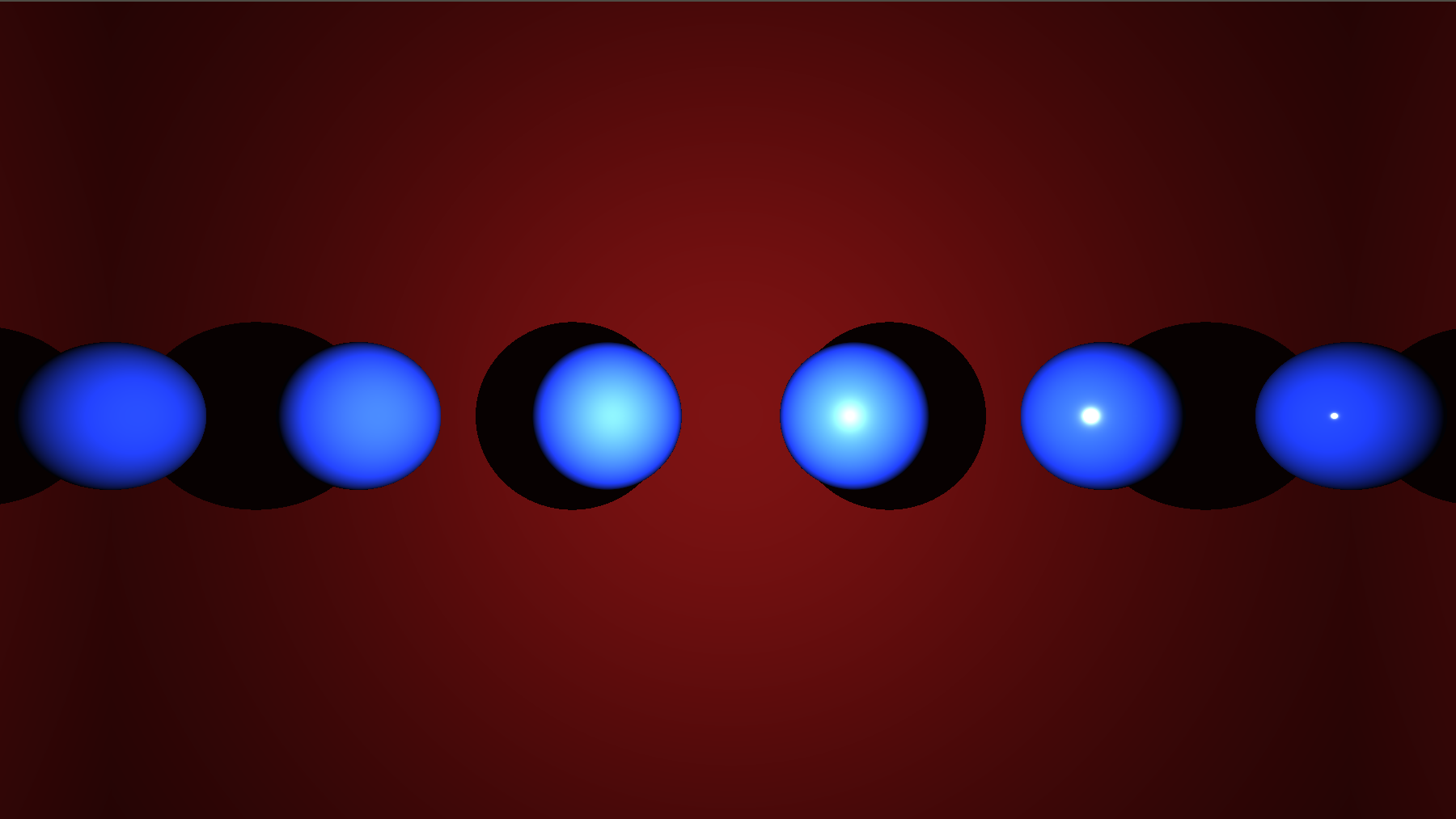
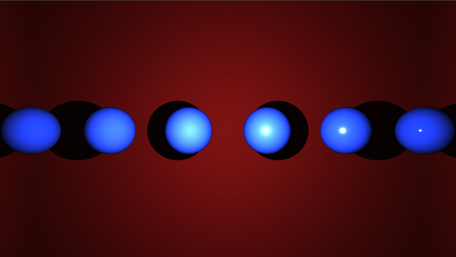
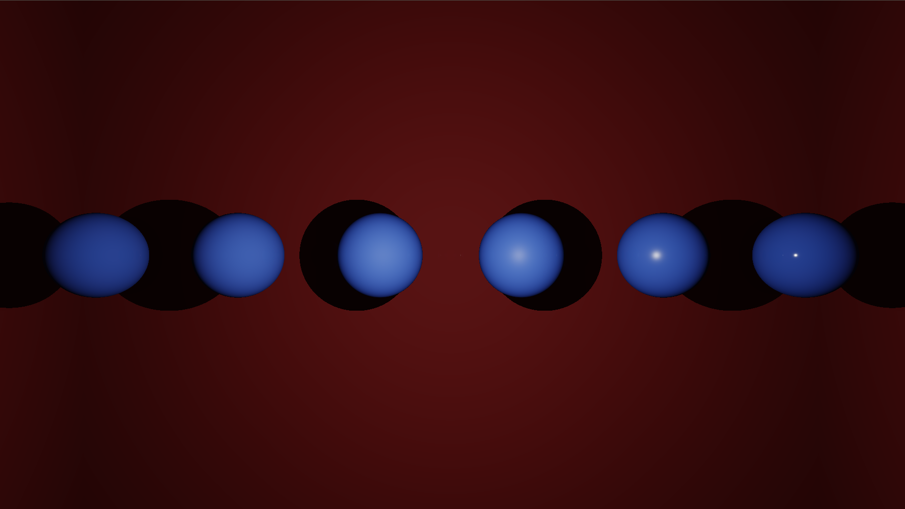
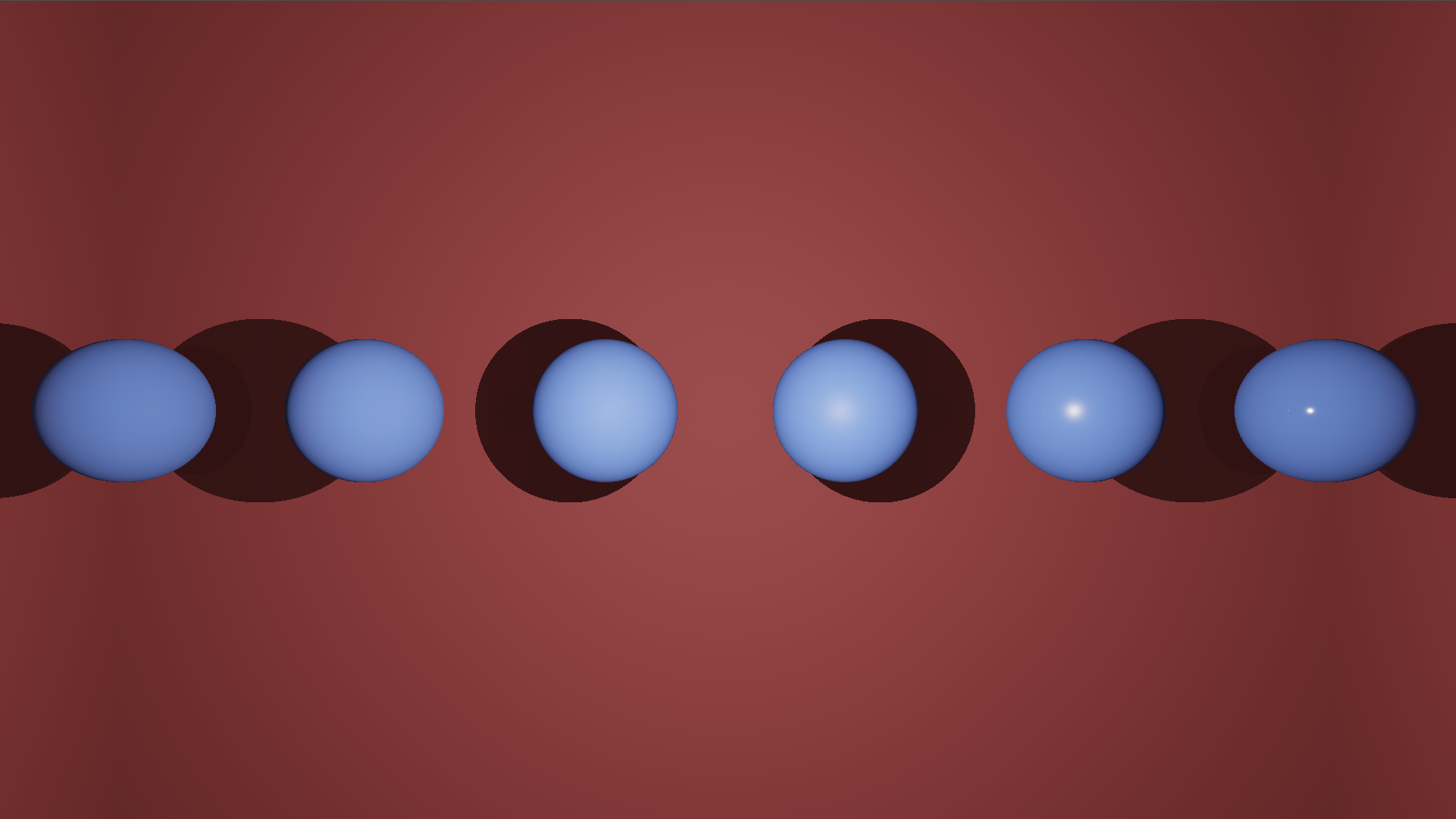
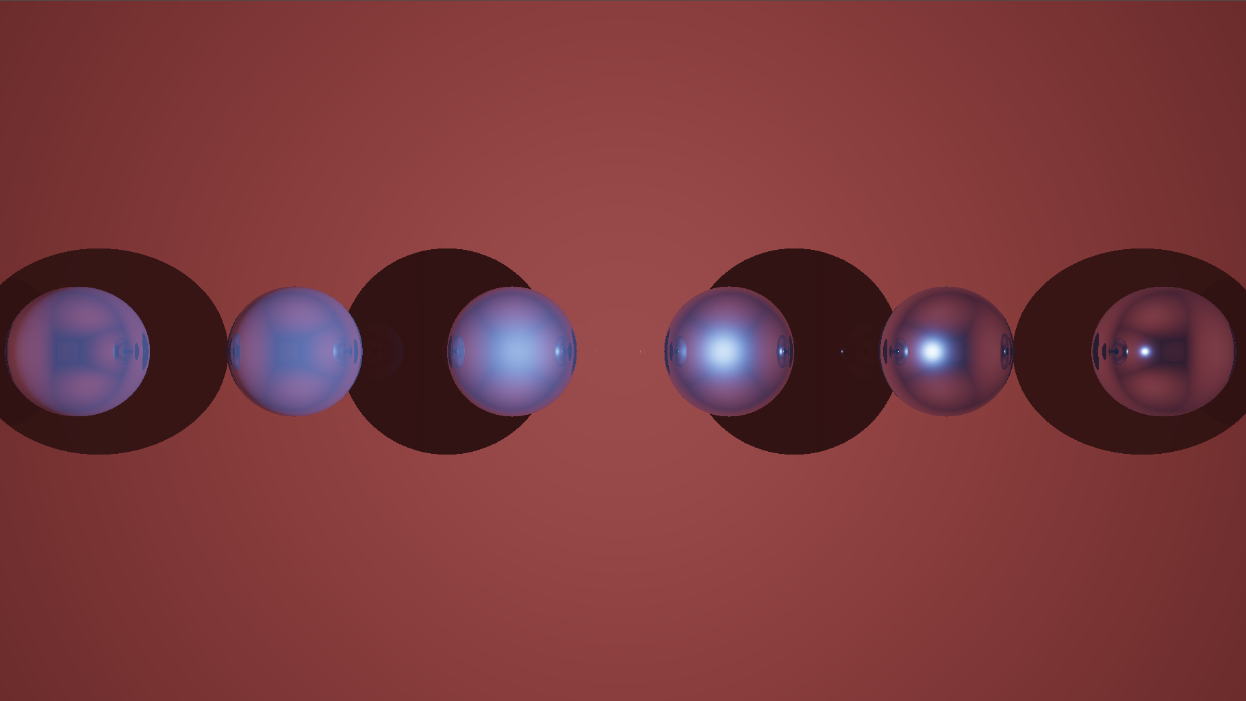
Here are the corrected images of the previous examples with different gamma values.

Dielectric materials with reflection (metalness = 0) HDR and Gamma = 1

Dielectric materials with reflection (metalness = 0) HDR and Gamma = 2.2

Metallic material with reflection (metalness = 1) HDR and Gamma = 1

Metallic material with reflection (metalness = 1) HDR and Gamma = 2.2

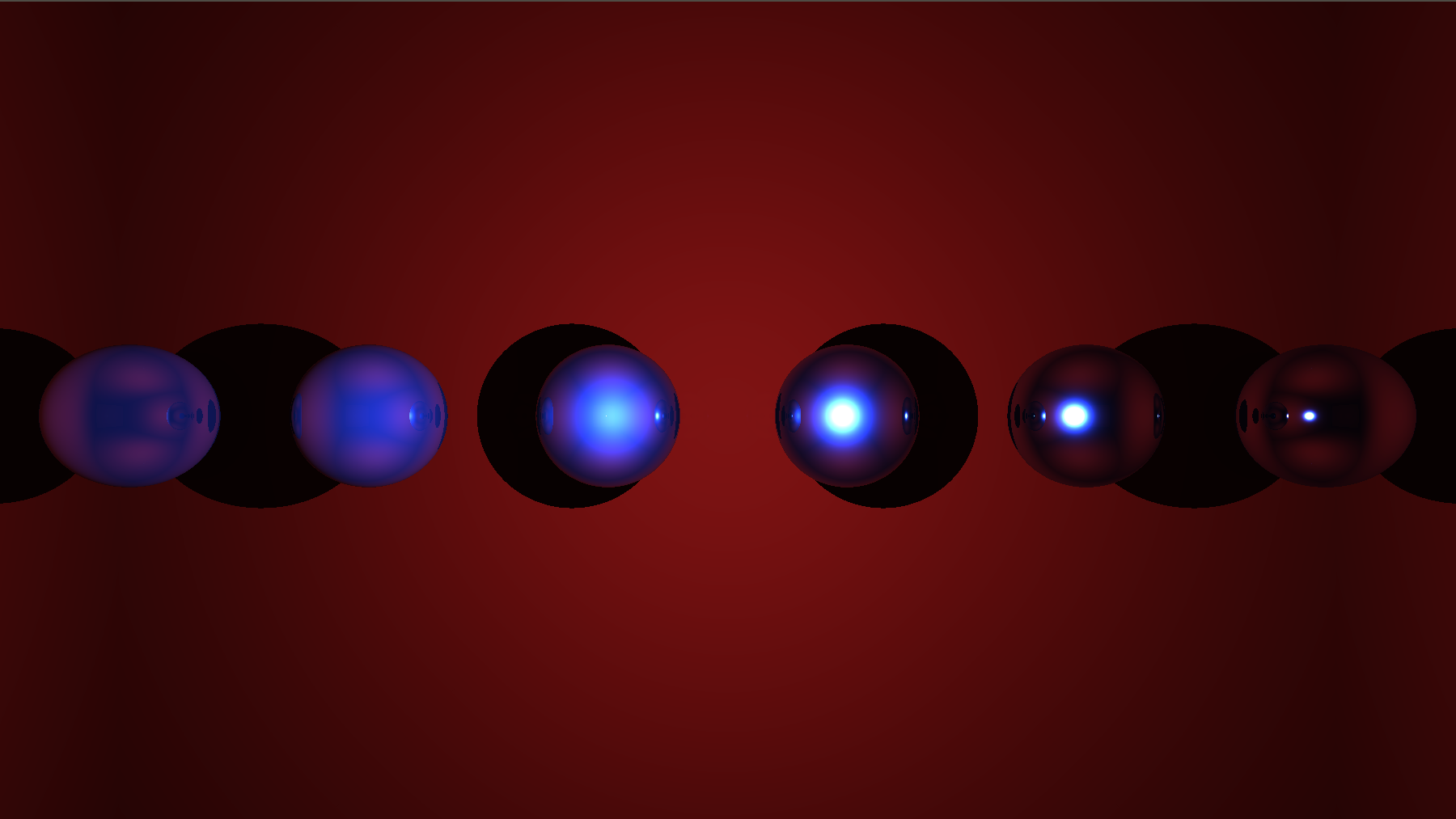
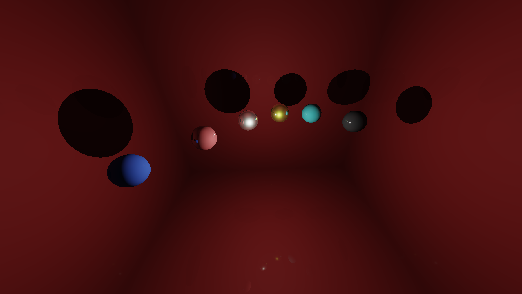
You can also play with the different parameters and get various materials:

And then ? What’s Next ?

Rendering is a huge topic and we covered a very small part of it. What is next entirely depends on which direction you want to pursue this journey; you could go into path tracing and ignore real-time approximations or on the contrary go for more real-time rendering effects like Image Based Lighting (IBL), Screen Space Ambient Occlusion (SSAO), Screen Space Reflections (SSR) and so on.

However, There is one aspect that should be improved in our current raytracing context which is the way we handle reflections. Indeed, currently in our ray-tracing context we cast only one reflected ray from intersection point. While it is accurate to do so for smooth surfaces, it is totally wrong for rough surfaces as we should cast several rays from the each intersection point and average the results in order to get the blurred reflections like I mentioned at the beginning of the tutorial. This is something you could try to implement in a naive manner and see how reflections are improved. In addition, one can also questions the fact the presence of an ambient lighting term in this energy conservative context and he/she is right, this term is a complete hack to cope with the lack of indirect lighting computation. For real-time applications IBL can be used to better approximate this kind of lighting contribution while path tracing implicitly compute this contribution.

Finally, I want you to be aware that BRDF models are generalizable and can take into account more light dimensionality, in particular:

BTDF: Bidirectionnal Transmission Distribution Function 5D: Same as BRDF for opposite side of surface
SVBRDF: Spatially Varying BRDF 6D: changes over the surface position
BSSRDF: Bidirectionnal Surface Scattering DF 8D: light exits at another location
BSDF: Bidirectionnal Scattering Distribution Function XD: General formulation