An Introduction to Raymarching

Jan 1, 0001

This tutorial is part of the ray-tracing course available here. /!\ This tutorial is using parts of the PBR tutorial which should be completed before starting this one.

Introduction

In this tutorial, I will introduce another well known rendering approach which is very similar to ray tracing but operates in a slightly different way, especially as it treats surfaces as distance fields. Ray tracing is based on the principle that we can compute analytically ray-surface intersections, being with triangles or more complex surfaces. However, this can also be a limitation as we are bound to display only surfaces for which we are able to compute ray-surface intersection. Thus, Ray Marching comes into place and allows us to display any surface defined by an expression $f(x,y,z) = 0$ such that $\left\lVert \nabla f \right\rVert = 1$, in other words a distance field. More precisely, in our context the $f$ function can also represent negative distances. It is referred as a Signed Distance Function (SDF) which means that when $f(p) > 0$, $p = (x,y,z)$ lies outside the surface and when $ f(p) < 0 $ it lies inside the surface. Note the D for Distance in SDF which imposes the condition $\left\lVert \nabla f \right\rVert = 1$.

Main Principle

The main principle of Ray Marching remains similar to Ray Tracing: for each pixel of the screen, we cast a ray spreading from the camera center to the pixel, however instead of computing ray surface intersections by solving an equation, we iterate through the generated ray step by step and check if we intersect a surface at each step by evaluating the scene SDF at the current location. More precisely, for a given ray $r(t) = \vec{d}t + c_{camera}$ and a given surface, we compute the SDF of the surface $f(r(t))$ and check if it equals 0. If not, we increase $t$ by a given amount $\delta_t$. Note that $t = 0 $ at the beginning of this process and that $f(r(0))$ should be positive. In practice $f(r(t)) = 0$ never occurs in our programming world, instead we will check if $f(r(t)) \leq 0$ meaning that we went through the surface.

Note that each surface like a Sphere or a Plane defines its own SDF that represents the closest distance from any given 3D point $p$ to the surface. Ray Marching also gives us the opportunity to combine each SDF with different operators in order to build multiple scenes with the same surfaces. The basic operation being the union of a SDF : $$SDF_{scene} (p) = \bigcup SDF (p) = \min\limits_{f \in SDF}(f(p))$$ Several other operators are commonly used like the intersection, the substraction or the smooth union.

Union	Intersection	Substraction	Smooth Union

Marching

There are different ways of choosing the value of $\delta_t$ while going through a light ray: one is to increase $t$ by a constant small value until we intersect one surface. Another one is to compute the minimal distance we can travel without intersecting any surface by taking the minimum of all $f(r(t))$. In practice, this minimal distance is equal to $SDF_{scene}(r(t))$. This second approach is called Sphere (or Spherical) Marching and will be the approach we will use in this tutorial.

Once we computed the intersection point, we are ready to compute any lighting occuring at this point as well as casting new rays to simulate reflections or refractions.

Coding Time

Now that I introduced the theory behind Ray Marching it is time to dig into actual coding. Like in previous ray tracing tutorials, we are working inside a fragment shader displaying a simple quad perfectly fitting our window. For each pixel we cast rays from a virtual camera to the current pixel whose screen coordinates are given by the in variable $fragCoord$.

void main() 
{   
	Ray ray = generatePerspectiveRay(fragCoord);
	outColor = vec4(march(ray),1);

}

The march function computes color contribution for the principal the reflected rays similarly to the trace function of previous tutorials. As we are in a PBR context, it also performs tone mapping and gamma correction. The function that actually go through each ray and check intersections with the surfaces in the scene is the rayMarch function. More precisely it returns the minimal $f(r(t))$ among all the scene surfaces. Notice that the normal at the intersection point is computed as the gradient of the surface SDF (see SDF Gradient section).

vec3 march(in Ray r)
{
    vec3 accum = vec3(0.0f);
    vec3 mask = vec3(1.0f);
    int nb_refl = 0;
    float c_refl = 0.3;
    Ray curr_ray = r;
    for(int i = 0 ; i <= nb_refl ; i++)
    {
	ISObj io = rayMarch(curr_ray);
	if(io.t >= 0)
	{
	    PBRMat mat = PBRMat(vec3(.9,.1,.1),0.4,0.9,0.3);
	    vec3 N = normalize(computeSDFGrad(io,curr_ray.ro + io.d * curr_ray.rd));

	    HitSurface hs = HitSurface(curr_ray.ro + io.d*curr_ray.rd
	                               ,N
	                               ,mat
	                               ) ;
	    vec3 color = directIllumination(hs,curr_ray,c_refl);
	    accum = accum + mask * color;

	    mask = mask*c_refl;
	    curr_ray  = Ray(hs.hit_point + 0.05*hs.normal,reflect(curr_ray.rd,hs.normal));
	}
	else if(i == 0) //did not intersect anything
	{
	    accum = vec3(0.3,0.2,0.8);
	}

    }

    //HDR
    accum = accum / (accum+ vec3(1.0));
    //Gamma
    float gamma = 1.1;
    accum = pow(accum, vec3(1.0/gamma));

    return accum;
}

The directIllumination functions remains the same as presented in the PBR tutorial, the only change being for the function computing the shadow ray intersection.

vec3 directIllumination(in HitSurface hit,in Ray r,inout float refl)
{

    vec3 color = vec3(0);
    for(int i = 0 ; i < light_nbr ; i++)
    {
	Ray l_ray = lightRay(hit.hit_point,lights[i]);
	l_ray.ro = hit.hit_point + 0.01*hit.normal;
	ISObj io;

	io = rayMarch(l_ray);
	
	float d_light = lightDist(hit.hit_point,lights[i]);

	if(io.t < 0 || (io.t >= 0 && (io.d >= d_light)))
	{
	    color += PBR(hit,r,lights[i]);
	}
	else
	{
	    color +=  vec3(0.03) * hit.material.color * hit.material.ao;
	}


	vec3 Ve = normalize(r.ro - hit.hit_point);
	vec3 H = normalize(Ve + l_ray.rd);
	refl = length(fresnelSchlick(max(dot(H, Ve), 0.0),  mix(vec3(0.04), hit.material.color, hit.material.metallic)))*hit.material.ao;
    }

    return color;
}

Lets detail the rayMarch function then. We first declare a maximum number of iteration step, defining how many times we can advance in the same ray. Indeed passed this number or a maximum travel distance we consider that nothing is to be intersected by the ray. Elsewise, at step $i$ we define the current point on the ray as $p = r.ro + depth * r.rd$, $depth$ playing the role of our parameter $t$ as explained above. We then compute the scene SDF, at point $p$, composed of one or several primitive surfaces like spheres, planes and boxes. This function returns the distance to the closest surface at point $p$. If this distance is lower than a given epsilon ($march accuracy$) or negative we consider that the current $p$ is the intersection point with the scene, else we continue to iterate over the ray and either increase $depth$ by the closest distance (Spherical Marching) or by a fixed amount.

ISObj rayMarch(in Ray r)
{
    int nb_step = 300;

    float depth = 0.0f;
    float march_accuracy = 0.001;
    float march_step_fact = 0.01;

    for (int i = 0; i < nb_step; i++)
    {
	ISObj io = sceneSDF(r.ro + depth * r.rd);
	if (io.d <= march_accuracy)
	{
	    return ISObj(depth,io.t,io.i);
	}

	// Move along the view ray
	//Spherical Marching
	depth += io.d;
	// Step by Step Marching
	//depth += march_step_fact

	if (depth >= DIST_MAX)
	{
	    // Gone too far; give up
	    return ISObj(DIST_MAX,-1,-1);
	}
    }
    return ISObj(DIST_MAX,-1,-1);
    //return ISObj(depth,last_io.t,last_io.i);
}

Computing the scene SDF is highly correlated with the way we represent the scene. In the last tutorials, we represented the scene as an union of Spheres, Planes and other surfaces whose intersection with a ray has an analytic solution. As I mentioned earlier, in our context we can combine surfaces using different operators which will change the shape of the represented surface. Thus, we need to add a new wrapper that contains both surfaces and operators that we apply between them. We define a Shape structure containing the type of primitive surface it represents and its index in the corresponding array (of Sphere, Plane,…). The ShapeOp structure contains one Shape, the operation to apply and the index of the next ShapeOp with whom the operator will be applied. By default we consider that $next = -1$, meaning that no operation will be applied, marking the end of the chained list of operations between primitive surfaces. To be more flexible in the way we build scenes, we allow ourselves to consider as many ShapeOp chain lists as we want. Thus, we define define an array of indices $shop roots$ from which each chained lists of ShapeOp should start.

struct Shape
{
    int shape_type;
    int shape_id;
};

struct ShapeOp
{
    Shape shape;
    int op_type;
    int next;
};

const int shop_nbr = 1;
ShapeOp shops[shop_nbr] = ShapeOp[](ShapeOp(Shape(1,0),0,-1));

const int shop_root_nbr = 1;
int shop_roots[shop_root_nbr] = int[](0);

As a starter, let’s consider one simple scene composed of a unique Sphere. Below I put the necessary code to define the three primitives I use in this tutorial. Note that this code should be put before the code section presented just above.

const int plane_type = 0;
const int sphere_type = 1;
const int box_type = 2;
const int shop_type = 3;

// plane structure
struct Plane 
{
    vec3 n; // normal
    float d; // offset
};

// box structure
struct Box 
{
    vec3 b; // up_right_corner_length
    vec3 c; // center
};


// sphere structure
struct Sphere 
{
    vec3 c; // center
    float r; // radius
};

const int sphere_nbr = 6;

Sphere spheres[sphere_nbr] = Sphere[](Sphere(vec3(0.5,-2.5*cos(time*0.1),0),0.5f)
	,Sphere(vec3(0.7,-2.5*cos(time*0.2),0),0.5f)
,Sphere(vec3(0.9,-2.5*cos(time*0.3),0),0.5f)
,Sphere(vec3(-0.9,2.5*cos(time*0.4),0),0.5f)
,Sphere(vec3(-0.7,2.5*cos(time*0.5),0),0.5f)
,Sphere(vec3(-0.5,2.5*cos(time*0.6),0),0.5f));

const int box_nbr = 3;
Box boxes[box_nbr] = Box[](Box(vec3(1,1,1),vec3(0,-3,0)),Box(vec3(1,1,1),vec3(0,3,0)),Box(vec3(0.5,0.5,0.5),vec3(0,0,0)));

const int plane_nbr = 6;
Plane planes[plane_nbr] = Plane[](Plane(vec3(0,1,0),5.0f),Plane(vec3(0,-1,0),5.0f),Plane(vec3(0,0,1),5.0f),Plane(vec3(0,0,-1),15.0f)
,Plane(vec3(1,0,0),5.0f),Plane(vec3(-1,0,0),5.0f));

Lets now compute the scene SDF at the current ray point $p$ within the chained list of surface operators, defining a single sphere. We iterate through each chain list, compute their related SDF by iteratively applying SDF operators and returns the closest computed distance among all chained lists (only one in our case).

ISObj sceneSDF(in vec3 point)
{
    ISObj nearest = ISObj(DIST_MAX,-1,-1);
    for(int j = 0 ; j < shop_root_nbr ;j++)
    {
	float dist = ShapeSDF(shop_roots[j],point);
	if(dist < nearest.d)
	    nearest = ISObj(dist,shop_type,shop_roots[j]);
    }
    return nearest;
}

float ShapeSDF(int sh_op_id, vec3 p)
{
    int curr_id = sh_op_id;
    float sdf_f = getBasicSDF(shops[curr_id].shape.shape_type,shops[curr_id].shape.shape_id,p);
    int next_id = shops[sh_op_id].next;

    while(next_id != -1)
    {
	float sdf_i = getBasicSDF(shops[next_id].shape.shape_type,shops[next_id].shape.shape_id,p);
	sdf_f = OpSDF(sdf_f,sdf_i,shops[curr_id].op_type);
	curr_id = next_id;
	next_id = shops[next_id].next;
    }

    return sdf_f;
}

Eventually, we need to define the SDF of each primitive surfaces in $getBasicSDF$ as well as the surface operators in $OpSDF$.

float getBasicSDF(int type, int id,in vec3 p)
{
    if(type == plane_type)
    {
	    return SDFPlane(planes[id],p);
    }
    else if(type == sphere_type)
    {
	return SDFSphere(spheres[id],p);
    }
    else if(type == box_type)
    {
	return SDFBox(boxes[id],p);
    }

    return 0.0;
}

// signed distance function of sphere 
float SDFSphere(in Sphere s, in vec3 p) 
{
    return length(s.c - p) - s.r;
}

// signed distance function of plane 
float SDFPlane(in Plane pl, in vec3 p) 
{
    return (pl.d + dot(normalize(pl.n),p));
}

// signed distance function of Box 
float SDFBox(in Box b, in vec3 p) 
{
    vec3 d = abs(p - b.c) - (b.b) ;
    return length(max(d,0)) + min(max(max(d.x,d.y),d.z),0);
}


float OpSDF(in float s_sdf, in float e_sdf, int op_t)
{
    if(op_t == 0)
    {
	return opUnion(s_sdf,e_sdf);
    }
    else if(op_t == 1)
    {
	return opSubtraction(s_sdf,e_sdf);
    }
    else if(op_t == 2)
    {
	return opIntersection(s_sdf,e_sdf);
    }
    else if(op_t == 3)
    {
	return opSmoothUnion(s_sdf,e_sdf,1.0f);
    }

    return 0.0;

}

float opUnion( float d1, float d2 ) {  return min(d1,d2); }

float opSubtraction( float d1, float d2 ) { return max(d1,-d2); }

float opIntersection( float d1, float d2 ) { return max(d1,d2); }

float opSmoothUnion( float d1, float d2, float k ) 
{
    float h = clamp( 0.5 + 0.5*(d2-d1)/k, 0.0, 1.0 );
    return mix( d2, d1, h ) - k*h*(1.0-h);
}

SDF gradient

We are one step away of displaying our first ray marched scene. Indeed, the only unknown left to compute is the normal at the intersection point which is especially used to compute the local illumination. In this context, as we apply SDF operators, we will build new scenes by combining primitive surfaces in different ways. Consequently, we cannot compute an analytical normal at the intersection point. Instead we use finite differences to compute an approximation of this normal which correspond to the gradient of the scene SDF at this point. In the 1D case, approximating such a gradient (derivative) is done as following $f'(x) = \frac{f(x+\epsilon) - f(x - \epsilon)}{2\epsilon}$. As SDFs are 3D functions, this principle is extended to each dimension of the function: $$\nabla f = \frac{(f(p + (\epsilon,0,0)) - f(p - (\epsilon,0,0)), f(p + (0,\epsilon,0)) - f(p - (0,\epsilon,0)), f(p + (0,0,\epsilon)) - f(p - (0,0,\epsilon))) } {2(\epsilon,\epsilon,\epsilon)}$$

float getSDF(int type, int id,in vec3 p)
{
    if(type != shop_type)
    {
	return getBasicSDF(type,id,p);
    }
    else
    {
	return ShapeSDF(id,p);
    }
}


#define EPS_GRAD 0.001
vec3 computeSDFGrad(in ISObj is,in vec3 p)
{
    vec3 p_x_p = p + vec3(EPS_GRAD, 0, 0);
    vec3 p_x_m = p - vec3(EPS_GRAD, 0, 0);
    vec3 p_y_p = p + vec3(0, EPS_GRAD, 0);
    vec3 p_y_m = p - vec3(0, EPS_GRAD, 0);
    vec3 p_z_p = p + vec3(0, 0, EPS_GRAD);
    vec3 p_z_m = p - vec3(0, 0, EPS_GRAD);

    float sdf_x_p = getSDF(is.t,is.i,p_x_p);
    float sdf_x_m = getSDF(is.t,is.i,p_x_m);
    float sdf_y_p = getSDF(is.t,is.i,p_y_p);
    float sdf_y_m = getSDF(is.t,is.i,p_y_m);
    float sdf_z_p = getSDF(is.t,is.i,p_z_p);
    float sdf_z_m = getSDF(is.t,is.i,p_z_m);


    return vec3(sdf_x_p - sdf_x_m
	        ,sdf_y_p - sdf_y_m
	        ,sdf_z_p - sdf_z_m)/(2.*EPS_GRAD);
}

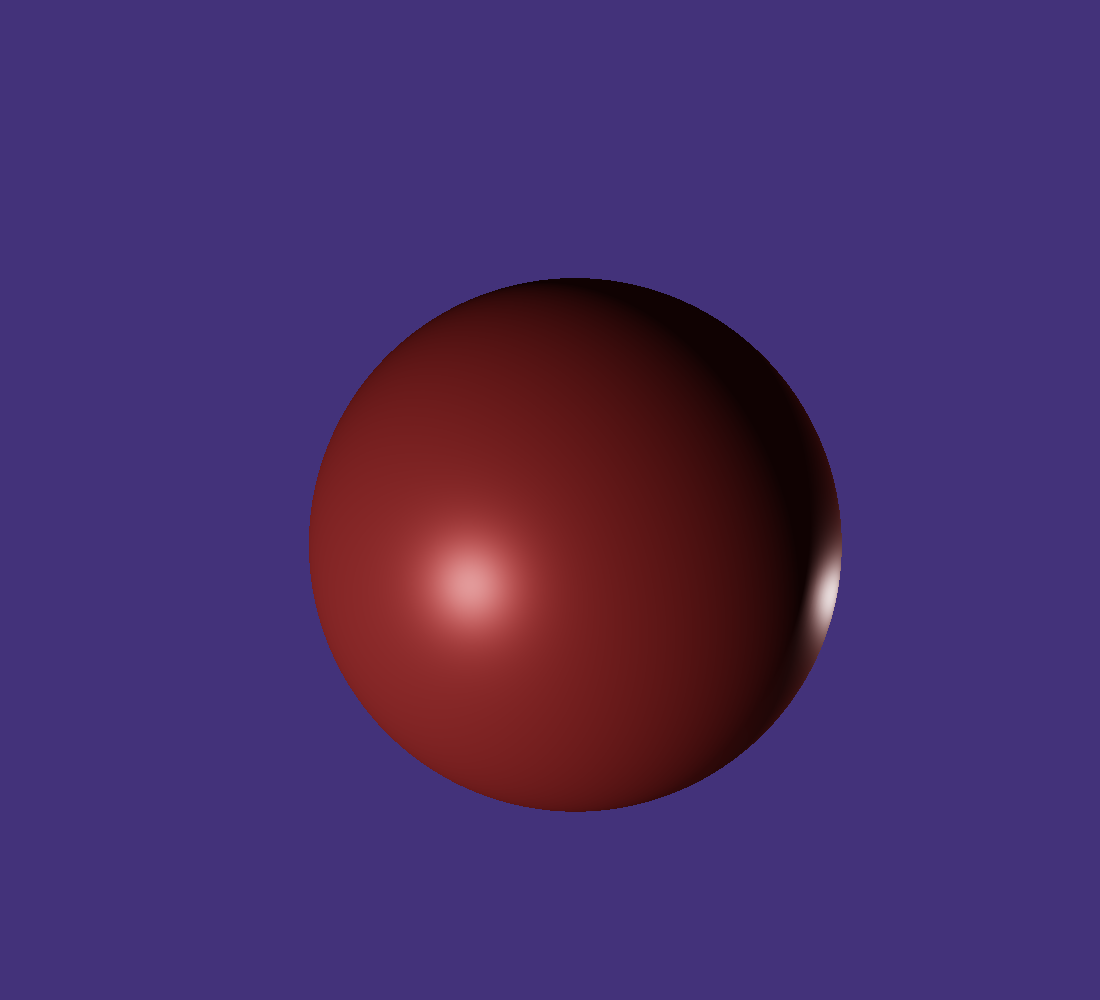
Using the following lights in your scene you should now obtain a correctly shaded ray marched sphere.

const int light_nbr = 2;
Light lights[light_nbr] = Light[](Light(1,vec3(1,1,-1),vec3(-3,1,-3),80,vec3(1))
	,Light(1,normalize(vec3(-1,1,1)),vec3(3,1,3),80,vec3(1)));

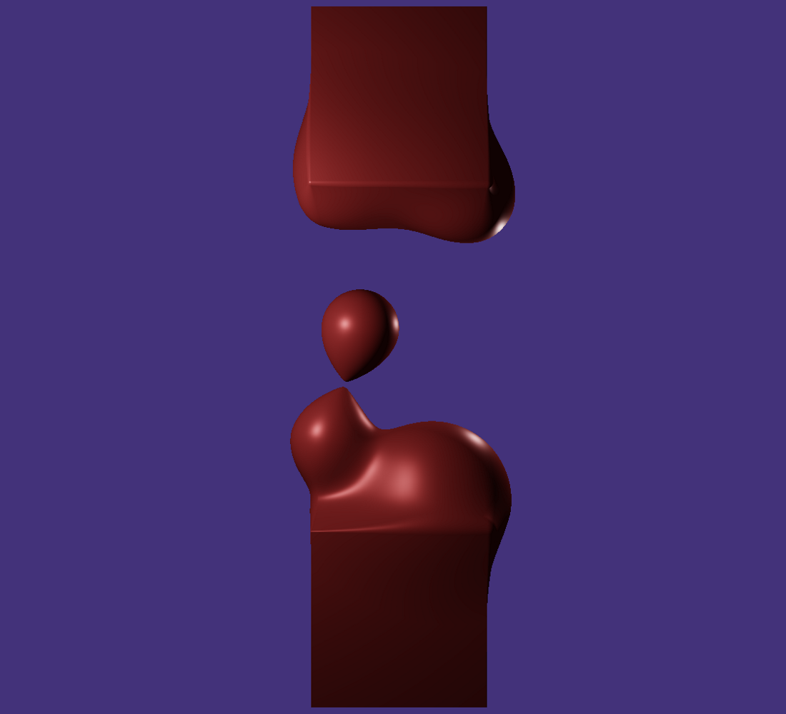
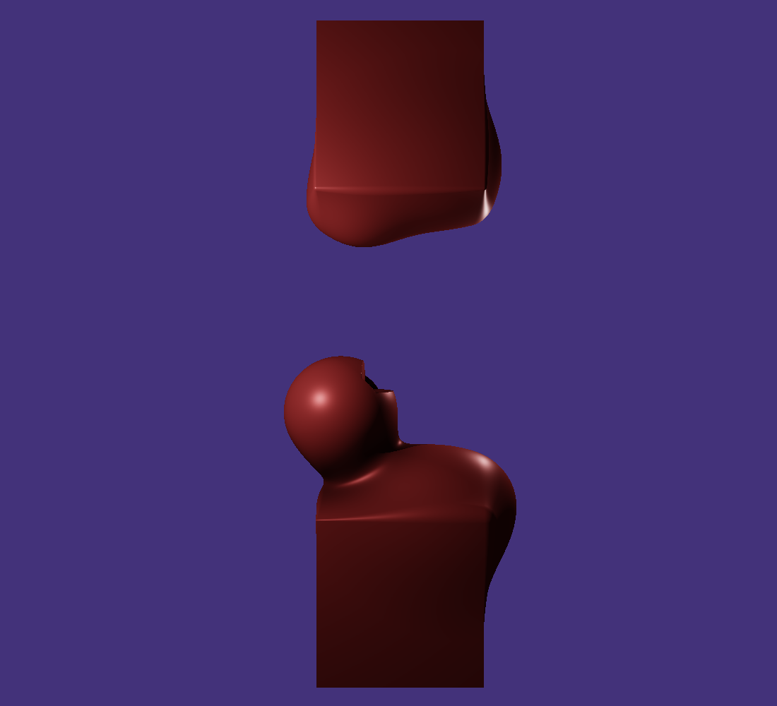
Example : March Lava Lamp

Let’s now build a more complex scene using only one ShapeOp chained list. The main idea here is to display a kind of lava lamp using spheres and two boxes. This can be easily achieved by using the smooth union operator which interpolates between two SDF that are near each other.

const int shop_nbr = 10;
ShapeOp shops[shop_nbr] = ShapeOp[](ShapeOp(Shape(1,0),3,1)
	,ShapeOp(Shape(1,1),3,2)
,ShapeOp(Shape(1,2),3,3)
,ShapeOp(Shape(1,3),3,4)
,ShapeOp(Shape(1,4),3,5)
,ShapeOp(Shape(1,5),3,6)
,ShapeOp(Shape(2,0),3,7)
,ShapeOp(Shape(2,1),1,-1)
,ShapeOp(Shape(2,2),1,-1)
,ShapeOp(Shape(0,0),0,-1));

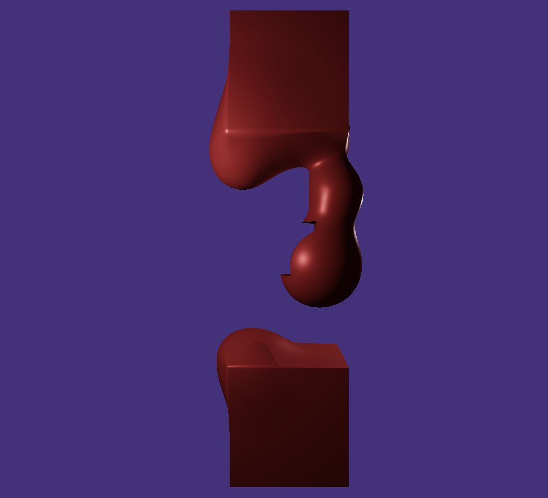
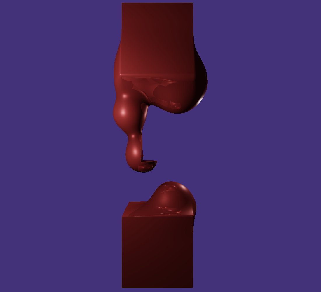
Lets also put a cube shaped hole inside this lamp using the substract operator.

const int shop_nbr = 10;
	ShapeOp shops[shop_nbr] = ShapeOp[](ShapeOp(Shape(1,0),3,1)
		,ShapeOp(Shape(1,1),3,2)
	,ShapeOp(Shape(1,2),3,3)
	,ShapeOp(Shape(1,3),3,4)
	,ShapeOp(Shape(1,4),3,5)
	,ShapeOp(Shape(1,5),3,6)
	,ShapeOp(Shape(2,0),3,7)
	,ShapeOp(Shape(2,1),1,8)
	,ShapeOp(Shape(2,2),1,-1)
	,ShapeOp(Shape(0,0),0,-1));

Now that you can render more complex scenes and I invite you to test all kind of scene configurations by playing with different primitives and different operators.

Bonus Effect: Ambient Occulsion

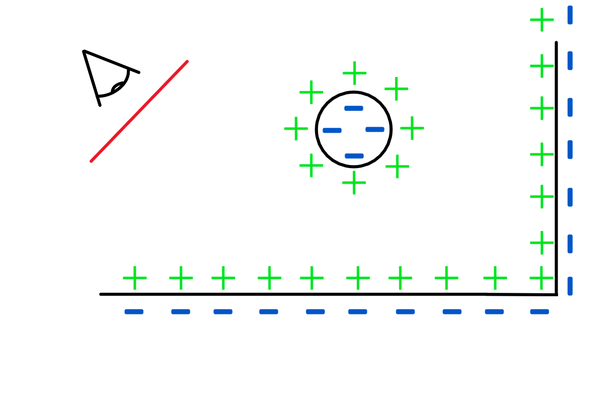
Rendering 3D scenes using ray marching also offer other advantages. Additional rendering effect like Ambient Occlusion can be computed with a reduced cost. Ambient Occlusion is the equivalent of ambient lighting but for shadowing, it describes which parts of the scene that are likely to not be lighted because of the geometry of its surroundings, preventing light ray to reach those areas. This effect can be simply be noticed at the edges and corners of your room where lights hardly strike those areas. Ray Marching offers us a simple way to approximate this ambient occlusion term. The main idea is to cast an ambient occlusion ray from the intersection point $p$ in the normal direction $\vec{n}$ and march through this ray step by step with a relatively small $\delta_t$. Then at each step, we compute the scene SDF and compare its value to the distance with respect to the intersection point which is equal to $i \delta_t$, $i$ being the number of the current step. In the case where the intersection point lies on a convex surface like a sphere we expect this distance and the scene SDF to be the same. However, it is far from being true in the general case, meaning that the scene SDF can be lower than $i \delta_t$ at some steps, being nearer to other surfaces. This simulate the fact that some areas around the intersection point can occlude incoming rays. In practice, we first initialize the occlusion factor at $1$ and compute at each step $\frac{(i \delta_t - SDF_{Scene})^2}{i}$ and subtract this amount to the occlusion factor. Notice the denominator which takes into account that the farther from the intersection point we make this evaluation the less plausible it is as we might look far from the surroundings.

float AmbientOcclusion(vec3 point, vec3 normal, float step_dist, float step_nbr)
{
    float occlusion = 1.0f;
    while(step_nbr > 0.0)
    {
	occlusion -= pow(step_nbr * step_dist - (sceneSDF( point + normal * step_nbr * step_dist)).d,2) / step_nbr;
	step_nbr--;
    }

    return occlusion;
}


vec3 march(in Ray r)
{
	...
	for(int i = 0 ; i <= nb_refl ; i++)
	{
		ISObj io = rayMarch(curr_ray);
		if(io.t >= 0)
		{
			...
			accum = accum + mask * color * pow(AmbientOcclusion(hs.hit_point,hs.normal,0.015,20),40);

			...
		}
		else if(i == 0) //did not intersect anything
		{
			accum = vec3(0.3,0.2,0.8);
		}

	}
	...

	return accum;
}

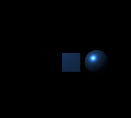
It is important to note that when computing the ambient occlusion term, the total travel distance should remain as short as possible because. Indeed, like mentioned earlier, the farther you travel through this ray, the more artifact you are likely to get because surfaces that are too far away from the intersection point might contribute to the occlusion term while not being part of its surroundings. With the parameters I used, you should have an ambient occlusion terms like depicted below. Note that I amplified its effect using a power function with a relatively high factor.

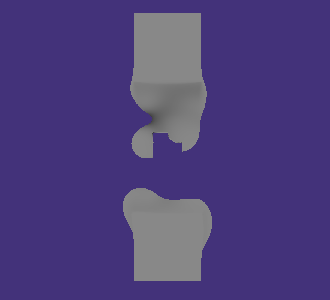
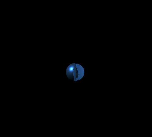
Below is what you should obtain by multiplying the ambient occlusion to the output color so that it plays a shadowing role.

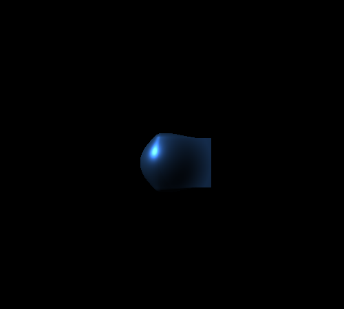
Finally, we can also re-enable relections in the main loop and get the following result.

What is next

This tutorial is a brief introduction to Ray Marching, there are still many things to cover. At least, three important aspects are to be studied, the first one being terrain marching, the second one fractal marching and the last one being the use of impostors in real-time rendering pipelines that are rendered using raymarching. In a future update, I will probably add a section about terrain marching, stay tuned.